Back-propagation with NumPy: From Tutorial to Line of Code 🧠

When Matt Mazur's 17-step tutorial becomes NumPy magic

Back-propagation powers Artificial-Neural-Networks(ANN) and its multi-hidden-layer version, Deep-Learning, basically “Artificial Intelligence” as we know IT. Been fascinated since i was working On identifying marker genes from gene expression data in a neural framework through online feature analysis which was an attempt to distinguish between two types of leukemia, acute myeloid and acute lymphoblastic types and eventually found a network consisting of a set of five genes that show 100% accuracy on the training set and 97.1% accuracy on the test

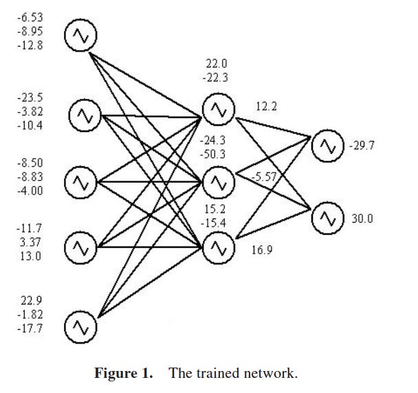
this gave us motivation to go forward with classifying even tougher problem of four heterogeneous childhood cancers with help from the creator of the algorithm, Shun'ichi Amari! Coding something like this from scratch took many lines of code though even though i was using PERL, lazy me like 🙃 quite hard to explain but thankfully found Matt Mazur's excellent backpropagation tutorial, where he walks through every single calculation step by step. It's incredibly detailed and educational, but still, lots of code 🫡 I couldn't help wondering: can we capture all that complexity in just a few lines of NumPy?

Spoiler alert: Yes! And the result is not just more concise - it's also more insightful. Let me show you how all those detailed calculations collapse into elegant matrix operations.

The Setup: A Simple but Revealing Network

neural network has a very specific configuration:

• Input: [0.05, 0.10]

• Hidden: 2 neurons with sigmoid activation [[0.15, 0.20], [0.25, 0.3]]

• Output: 2 neurons with sigmoid activation [[0.4, 0.45], [0.5, 0.55]]

• Target: [0.01, 0.99]

• Learning Rate: 0.5

• Constant Bias: [0.35,0.60]

Here's what the network looks like with all the initial weights and values:

Following is the update of network after first iteration

which matches the values in the original tutorial 🙏

AND after 10000 iterations, which is what we get with numpy version 🥳

SO what exactly is this code? First, let's install what we need:

pip install numpy

The Step-by-Step Implementation

Let me show you the no-loop version first - this is pure NumPy magic happening in just a few lines. Here's how I set up the network:

python

# Initial setup matching the network diagram above
inp=[0.05,0.10]                    # Input values
inpw=[[0.15,0.20],[0.25,0.3]]      # Input-to-hidden weights  
hidw=[[0.4,0.45],[0.5,0.55]]       # Hidden-to-output weights
outputr=[0.01,0.99]                # Target outputs
bias=[0.35,0.6]                    # Bias values for hidden and output
lr=0.5                             # Learning rate

import numpy as np
x=np.asarray(inp)
y=np.asarray(outputr)  
w1=np.asarray(inpw)    # Shape: (2,2) - from 2 inputs to 2 hidden
w2=np.asarray(hidw)    # Shape: (2,2) - from 2 hidden to 2 outputs

Now comes the forward propagation in two lines: python

# Hidden layer: sigmoid(inputs * weights + bias)
h=1/(1+np.exp(-(x.dot(w1.T)+bias[0])))
# h = [0.5932699921071872, 0.596884378259767] - hidden activations

# Output layer: sigmoid(hidden * weights + bias)  
y_pred=1/(1+np.exp(-(h.dot(w2.T)+bias[1])))
# y_pred = [0.7513650695523157, 0.7729284653214625] - predicted outputs

print(0.5*np.square(y_pred - y).sum())
# 0.298371108760003 - initial error

That initial error of 0.298371108760003 matches exactly what we expect from the tutorial! You can see how far our predictions [0.751, 0.773] are from our targets [0.01, 0.99].

The Backpropagation Magic ✨

Here's where it gets beautiful. All those detailed gradient calculations from the tutorial collapse into two elegant NumPy operations:

python

# Update output weights (w2) - captures all the ∂E/∂w calculations
w3=w2-lr*np.outer((y_pred - y)*(1-y_pred)*y_pred,h)

# Update input weights (w1) - captures all the chain rule complexity
w4=w1-lr*np.outer(w2.T.dot((y_pred - y)*(1-y_pred)*y_pred)*h*(1-h),x)

But why does, for example, np.outer((y_pred - y)*(1-y_pred)*y_pred,h) work? Let's break down the mathematics:

The Mathematical Beauty Behind np.outer()

For the output layer weights, we need to compute ∂E/∂wᵢⱼ for each weight connecting hidden neuron i to output neuron j.

From calculus and the chain rule:

∂E/∂wᵢⱼ = ∂E/∂outⱼ × ∂outⱼ/∂netⱼ × ∂netⱼ/∂wᵢⱼ

Let's compute each term:

1. ∂E/∂outⱼ = (outⱼ - targetⱼ) = (y_pred - y)

2. ∂outⱼ/∂netⱼ = outⱼ × (1 - outⱼ) = y_pred * (1 - y_pred) (sigmoid derivative)

3. ∂netⱼ/∂wᵢⱼ = hᵢ = h (the hidden layer activation)

So: ∂E/∂wᵢⱼ = (y_pred - y) × y_pred × (1 - y_pred) × h

Now here's the NumPy magic: we need this gradient for ALL combinations of i and j:

• For each output neuron j: multiply (y_pred - y) * y_pred * (1 - y_pred)

• By each hidden activation hᵢ

This is exactly what np.outer() does! It computes the outer product:

python

# If y_pred - y = [δ₁, δ₂] and h = [h₁, h₂], then:
np.outer([δ₁*(1-out₁)*out₁, δ₂*(1-out₂)*out₂], [h₁, h₂])
# produces:
# [[δ₁*(1-out₁)*out₁*h₁, δ₁*(1-out₁)*out₁*h₂],
#  [δ₂*(1-out₂)*out₂*h₁, δ₂*(1-out₂)*out₂*h₂]]

Each element [i,j] contains exactly ∂E/∂wᵢⱼ - the gradient for the weight from hidden neuron i to output neuron j!

Why This Is Brilliant

Instead of computing each ∂E/∂w₅, ∂E/∂w₆, ∂E/∂w₇, ∂E/∂w₈ separately (as in the tutorial), np.outer() computes ALL gradients simultaneously using vectorized operations. It's the same mathematics, but expressed in the language of linear algebra rather than individual scalar calculations.

That's it! Two lines that capture:

• All the partial derivatives (∂E/∂w₅, ∂E/∂w₆, ∂E/∂w₇, ∂E/∂w₈)

• All the chain rule applications (∂E/∂out₁ × ∂out₁/∂net₁ × ∂net₁/∂w)

• All the hidden layer gradient propagation

After one iteration:

python

h1=1/(1+np.exp(-(x.dot(w4.T)+bias[0])))
y_pred_h1=1/(1+np.exp(-(h1.dot(w3.T)+bias[1])))
print(0.5*np.square(y_pred_h1 - y).sum())
# 0.291027773693599

Perfect! We get 0.291027773693599, exactly matching the expected result from the tutorial.

The Network After Learning 🎯

Here's how the network looks after one backpropagation step:

[See the second Mermaid diagram above showing the updated weights and improved error]

Notice the fascinating changes:

• Input-to-hidden weights decreased slightly (learning to reduce the overall activation)

• Hidden-to-output weights had mixed changes: w5 and w6 decreased significantly, while w7 and w8 increased

• Total error dropped from 0.2984 to 0.2910 - that's learning in action!

• Output predictions moved closer to targets: o1 went from 0.7514 → 0.7421 (getting closer to 0.01), o2 went from 0.7729 → 0.7753 (getting closer to 0.99)

The weight changes tell a story: the network learned that to get o1 closer to 0.01 (much lower), it needed to reduce the weights from both hidden neurons to o1. For o2 to get closer to 0.99 (slightly higher), it made nuanced adjustments.

The Plot Twist: Extending to Multiple Iterations

The beauty of this NumPy approach is that we can easily extend it to multiple iterations. Here's how you can run the same logic for any number of iterations:

for iteration in range(iterations):
    # Forward pass
    h = 1/(1+np.exp(-(x.dot(w1.T)+bias[0])))
    y_pred = 1/(1+np.exp(-(h.dot(w2.T)+bias[1])))
    error = 0.5*np.square(y_pred - y).sum()
    # Original implementation: parallel weight updates (same as no-loop version)
    # Calculate both updates using original weights
    w2_update = lr*np.outer((y_pred - y)*(1-y_pred)*y_pred, h)
    w1_update = lr*np.outer(w2.T.dot((y_pred - y)*(1-y_pred)*y_pred)*h*(1-h), x)
    # Apply updates in parallel
    w2 = w2 - w2_update
    w1 = w1 - w1_update

Expected output:

python ann_numpy_original.py 10
Iteration 1: Error = 0.2983711088
Iteration 10: Error = 0.2288087405
Expected Output:
[0.01 0.99]
Predicted Output:
[0.64517373 0.79406246]
Final Error: 0.22091859205390404

The network steadily learns, reducing error from ~0.29 to 0.22 over 10 iterations!

Why This Matters

This NumPy implementation teaches us something profound: complex mathematical operations can often be expressed elegantly through matrix operations. What takes Matt Mazur 17 detailed steps to explain becomes two lines of NumPy code that capture the exact same mathematical relationships.

But here's the key insight: the tutorial's step-by-step approach is invaluable for understanding what's happening, while the NumPy implementation shows us how to do it efficiently. You need both perspectives to truly master neural networks.

The matrix operations also reveal patterns that aren't obvious in the step-by-step approach:

• np.outer() naturally handles the broadcasting needed for gradient calculations

• The chain rule becomes matrix multiplication: w2.T.dot(...)

• Vectorization eliminates all the individual neuron calculations

Running the Full Implementation

You can explore the complete implementation:

bash

# Step-by-step (2 iterations only, matches tutorial exactly)
python ann_numpy_no_loop.py

# Extended version (any number of iterations)
python ann_numpy_original.py 10

I've also included analysis and visualization tools:

# Generate comparison analysis
python analyze_convergence.py

# Visualize the learning process
python plot_convergence.py

The Takeaway

This exploration taught me that there's incredible beauty in the relationship between detailed mathematical understanding and elegant implementation. Matt Mazur's tutorial gives you the deep understanding of why each calculation matters, while NumPy gives you the tools to express that same mathematics concisely and efficiently.

The two lines of backpropagation code aren't just shorter - they're also more generalizable. Once you see the pattern np.outer((error_signal) * (activation_derivative), input), you can apply it to networks of any size.

Plus, there's something deeply satisfying about seeing all those individual partial derivatives collapse into matrix operations. When you see np.outer((y_pred - y)*(1-y_pred)*y_pred,h) and realize that's computing gradients for your entire output layer - that's beautiful!

What's Next?

Try running the code yourself! The complete repository includes both the step-by-step implementation and the extended multi-iteration version, different way of updating, like sequential (turns out to converge just a little faster?) and multiple frameworks like jax/pytorch/tensorflow with auto-differentiation (explore GPU?), AND even language, C#!

Probably start with the tutorial to understand the mathematics, then appreciate how NumPy lets you express that same math elegantly. It's a perfect example of how the right abstractions can make complex operations both simpler and more powerful.

Have you found similar elegant expressions for complex mathematical operations? The journey from understanding to implementation is always fascinating!

---

All the code, analysis tools, and visualizations are available in the GitHub repository courtesy https://kiro.dev/. Feel free to experiment and see what insights you discover! 😊

---

fuzzyLife is a reader-supported publication. To receive new posts and support my work, consider becoming a free or paid subscriber.