
False discovery rating
Adjusting p-values the Benjamini & Hochberg way, a Million-Dollar Method!

The False Discovery Rate (FDR) method won the 2024 Rousseeuw Prize for Statistics - a million-dollar award recognizing outstanding statistical innovations that profoundly impact society. The laureates are Yoav Benjamini, Daniel Yekutieli, and Ruth Heller from Tel Aviv University, building on the groundbreaking 1995 paper by Benjamini and the late Yosef Hochberg (BH). Their research led to a method that limits false discoveries without stifling the potential for true discoveries. And the beautiful thing? It’s so simple you can do it in Excel and IT is my bread and butter! Something i “nudge” students to try cos i feel an Excel-lent way to learn something is to “reinvent the wheel” in Excel 🤞
tl;dr, Sort p-values → rank them → multiply each p-value by the total number of tests → divide by its rank.
So, let’s start
Uploaded excel sheet showcases this Million-dollar method in one Excel formula 🎯 I know IT is quick&dirty but your p-values via excel t.test function call, are already there and if you are layz as me, probably don’t want to switch tools 🙃 AND maybe you want to learn what is actually going on 🤓 so here are the steps
Step 1: Sort your p-values from smallest to largest
Step 2: Create a Rank column (1, 2, 3, ..., m) where 1 is smallest p-value to largest “m” which should also reflects total number of tests/p-values
Step 3: Fix cell containing “m” from Step 2, the excel way by adding $ to cell, $G$12 in this case
Step 4: Formula for the BH adjusted p-value:
=F2*$G$12/G2
Where:
F2= your p-value (changes for each row)$G$12= total number of tests (fixed with $)G2= rank (changes for each row)
This is literally the formula: BH_adjusted_p_value(i) = original_p_value(i) * (total_ranks)/(p_value(i)_rank), that’s IT!
Pro tip: If you have NaN or missing p-values, Excel will show #DIV/0! for those rows - that’s fine! Just means you can’t calculate FDR either because of the missing data (trŧ to replace NaN with literally ““ i.e. nothing) or too few values (more samples?) but still give unique rank to them for this to work 🤞
Double pro tip: Adjusted p-values must be monotone non-decreasing with rank.
Excel’s naive computation does not enforce this → you must fix it manually or for example by using =MIN(...) after calculating rank-based value because if a higher-ranked hypothesis has a smaller adjusted p-value than a lower-ranked one, the BH proof no longer holds 🫡 In our Excel sheet for example:

=MIN(I3, H2)My preferred way is to start from the highest p-values (bottom) and then copy this formula from penultimate row upwards, where H is your adjusted/calculated p-value column. This ensures no adjusted p-value is smaller than the one above it.

Following KISS principle, start with the simple formula of course and eyeball obtained values - if you see any adjusted p-value smaller than the previous one, use the previous one’s value instead. For most datasets this probably won’t matter but in this case without monotonicity constraint:
Position 1: (11/1) × 0.00071993 = 0.00791923
Position 2: (11/2) × 0.001390152 = 0.00764584 ← smaller!
Position 3: (11/3) × 0.001620303 = 0.00594111 ← even more so!
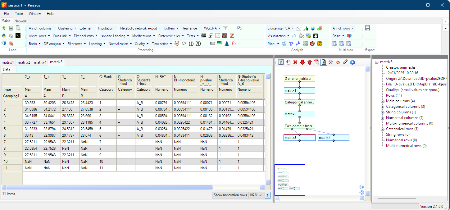
end up having position 3 is smaller than positions 1 and 2? That violates the monotonicity rule! This issue is something i found in https://groups.google.com/g/perseus-list/c/p5wgxzduBZQ/m/Rp7AvCuGAQAJ while using one of the most popular tools in proteomics (Perseus) and eyeballing results, the example shares here actually comes from that https://groups.google.com/g/perseus-list/c/EZUnI-j4W6Q/m/W2UCx4iv1dAJ issue! Hard to believe almost a decade has past but glad the issue is now fixed in Perseus 👌
The Python way (when you want automation with other python-based tools, AI?)
Python scipy.stats provides FDR correction function so adjusting p-values is a straightforward import and function call:
from scipy.stats import false_discovery_control
import numpy as np

# Your p-values
p_values = np.array([
    0.000719929,
    0.00139014,
    0.00162029,
    0.0146431,
    0.0147919,
    0.0263679,
    1, 1, 1, 1, 1
])

# Calculate FDR using Benjamini-Hochberg
fdr_values = false_discovery_control(p_values, method=’bh’)
print(f”FDR values: {fdr_values}”)
Output matches 🤞
FDR values: [0.00594106 0.00594106 0.00594106 0.03254218 0.03254218 0.04834115
 1.         1.         1.         1.         1.        ]
Finally, the R way cos statistical toys R us 👌
so of course, R has this built in natively:
pv<-c(0.00071993,0.001390152,0.001620303,0.014643094,0.014791889,0.026367867,1,1,1,1,1)

p.adjust(pv,method=”BH”)
 [1] 0.005941111 0.005941111 0.005941111 0.032542156 0.032542156 0.048341089 1.000000000 1.000000000 1.000000000 1.000000000 1.000000000
The p.adjust() function with method = “BH” is the canonical implementation and what everyone uses by default. Simple, battle-tested, works. At least the values match 👌 Actually this is what i end up using now a days cos i must admit that for huge data/tables, calculating all this in “Excel felt like drudgery” 🤪
Note
Original procedure:
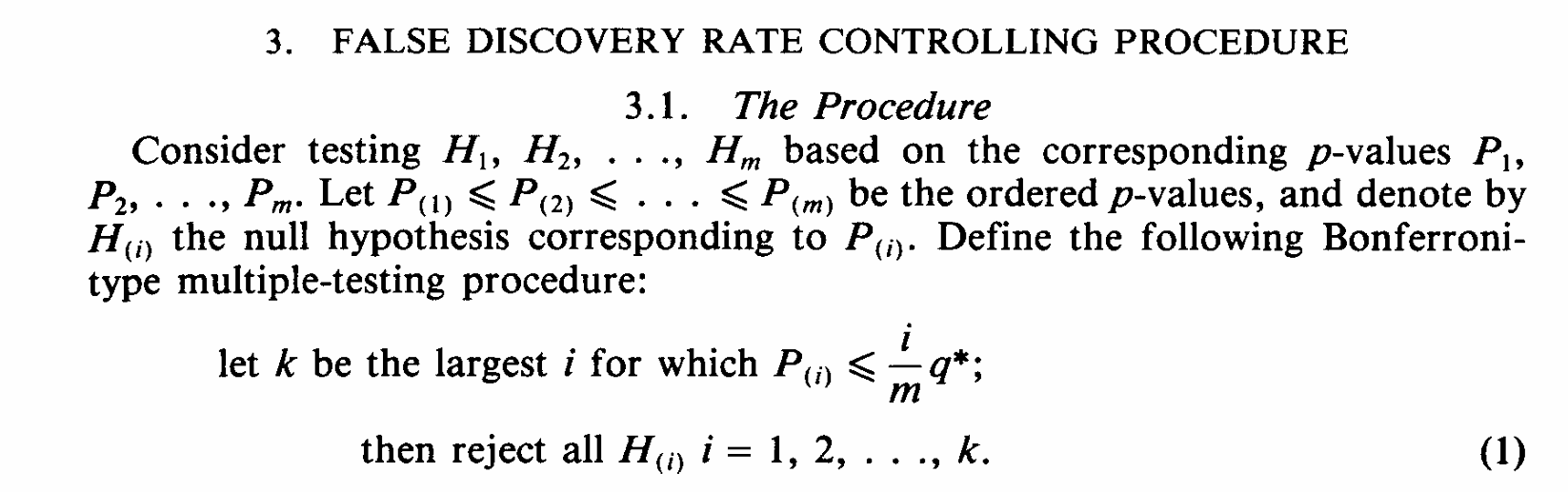
Takes your raw p-values and orders them: P(1) ≤ P(2) ≤ ... ≤ P(m)
Finds the largest rank i where P(i) ≤ (i/m) × q*
Rejects all hypotheses from rank 1 through i
Controls False Discovery Rate (expected proportion of false positives among rejections)
Why the transformation? The original BH paper says: P(i) ≤ (i/m) × q*
But software reports “adjusted p-values” which flip it to: (m/i) × P(i) ≤ q*
These are mathematically identical (just multiply both sides by m/i), but the second form is easier to use - for example to compare ALL adjusted p-values to ONE threshold (infamous~0.05) instead of comparing each raw p-value to DIFFERENT thresholds.
Example:
Original: Is 0.0146431 ≤ (4/11) × 0.05 = 0.01818? → YES
Adjusted: Is (11/4) × 0.0146431 = 0.04016 ≤ 0.05? → YES
Same answer, simpler comparisons/workflow!
Why this matters
In 1989, Branko Soriç warned that by ignoring multiple testing and focusing on selected discoveries, “a large part of science may be false.” Benjamini and Hochberg realized that the proportion of false discoveries among statistical discoveries could serve as a criterion for selection, rather than merely a warning.
Their insight: in a study with 100 genes, if you make 60 discoveries and 3 are false (5% FDR), that’s acceptable. But if you make 5 discoveries and 3 are false (60% FDR), that’s unacceptable. Not to mention

Power comparison
When ALL null hypotheses are true: FDR = FWER (same thing)
When SOME are false: FDR < FWER (more power with FDR!)
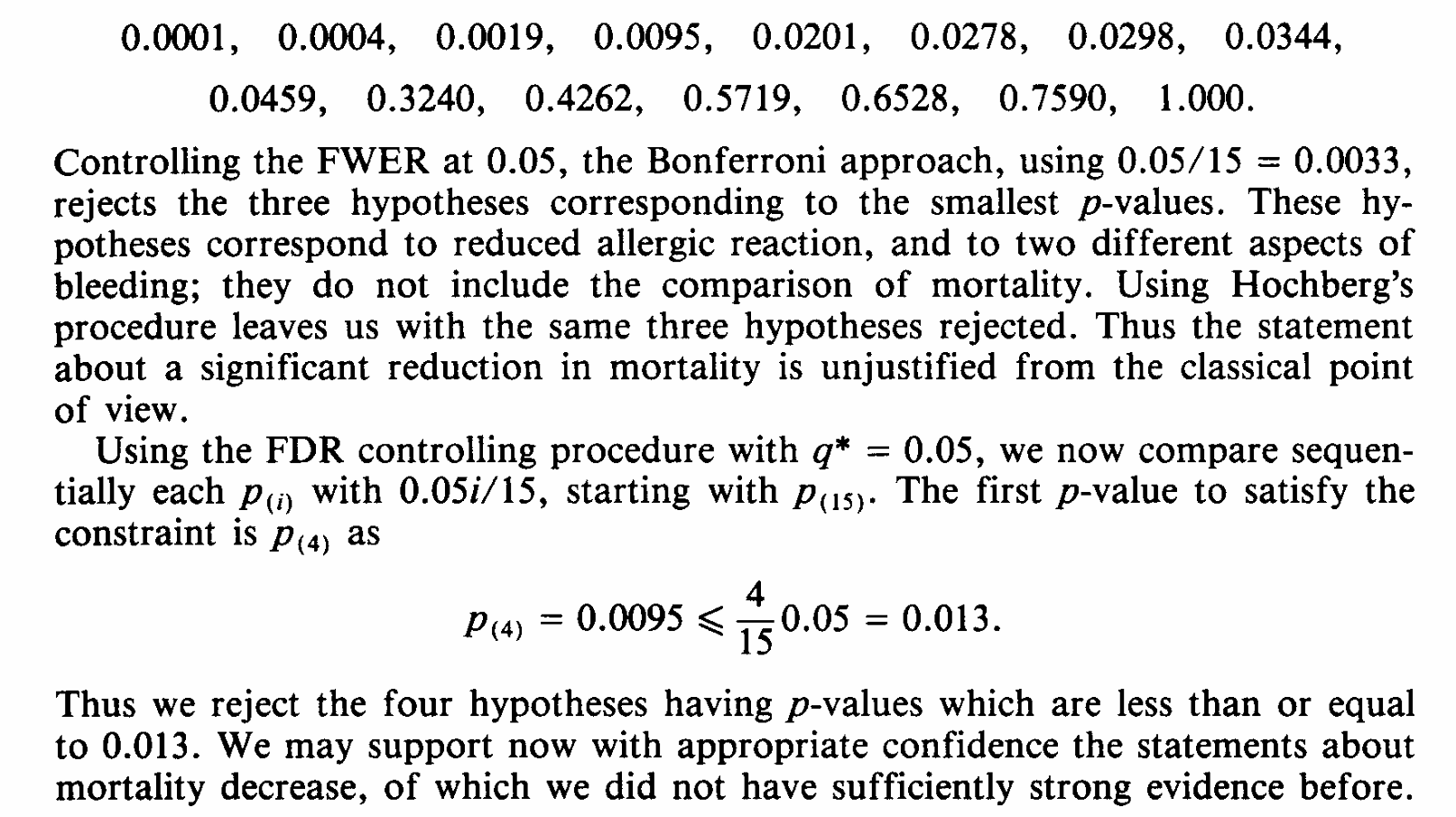
The original paper has this medical example: testing 15 endpoints in a thrombolysis trial. Using Bonferroni at α = 0.05, you’d use 0.05/15 = 0.0033 as threshold and reject 3 hypotheses. Using BH-FDR, you reject 4 hypotheses including the mortality comparison (p = 0.0095). That’s probably a real clinical impact though i must mention that guidelines for “preclinical“ Ischemia are not as clear, not to me at least 🫡
Limitations
Assumes independence of tests
Controls expected proportion of false discoveries, not probability of ANY false discovery
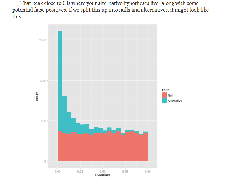
When studying this, be appropriately skeptical of results from fields prone to p-hacking, don’t forget to check p-value distribution http://varianceexplained.org/statistics/interpreting-pvalue-histogram/ for example
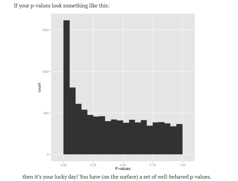
so it’s “probably” OK and further


Although FDR ≠ probability a discovery is false, beauty of FDR lets you make more discoveries while controlling the expected proportion of mistakes 🤞 for exploratory analysis, screening, genomics, or any situation where you care about the rate of false positives among your findings (not just whether ANY false positive occurred), FDR is probably what you want. And this method is so simple, one stepwise formula in Excel… sometimes even application of simple methods with solid theory can win you a million-dollar prize not to mention the method itself is a winner!
Let’s explore and find and/or apply more of these gems from our mathematical nature, and change the way “Science” is done/applied and probably win hearts and millions, wish you all the best 🥳