Learning LIMMA

by Rebuilding essential core From R to Python 🤞

Some statistical methods become so widely used that we don’t bother to check their internal structure! Linear-Models-for-Microarray-Data (limma) is one of them, abused extensively, especially in rna-seq-analysis 🙃 Basically limma is one of those R packages that has been quietly running inside almost every RNA-seq and microarray pipeline for 20+ years, even the follow-up Ritchie et al. 2015 paper has thousands of citations!! All in just two lines of R:

fit <- limma::lmFit(data,annotation)
fit <- limma::eBayes(fit)

AND suddenly small-sample variance begets “power”. But there is no magic thanks to the fact that the code is open-source, just

git clone https://git.bioconductor.org/packages/limma

Moderated t-statistics appear and things look&feel more “sciency” with fancierr t-test, my bread and butter 🙏

Basic Differential Expression Analysis App

cos proteomics data is way messier, missing values, HUGE range… limma has become limpa to deal with all that but so far it gives terrible results on our data 💩 maybe it is just me but hoping a fix from AI overlords soon, post will follow 🤞

Ani-ways digging deeper into limma, what we see is that something like moderating/shrinkage variance is going on with something called empirical Bayes. Now don’t ask me how can Bayes be not “empirical”🤪 I will leave that exploration for some other time, this post documents is an attempt to rebuild that engine from scratch, at least core of it, in a single python script, of course with copilot/chatGPT+claude 🙏 Given the source code, got quite close just over few hours!

Essentially generate some data with R script gen_input.R

curl https://raw.githubusercontent.com/animesh/scripts/650a951acf8fbe3a38bac6611b474eeac39bc63e/gen_input.R > gen_input.R 

for example and

Rscript.exe gen_input.R

Usage: Rscript scripts/gen_input.R [seed] [ngenes] [nA] [nB] [maxval]
  seed   : integer (default 1)
  ngenes : integer, number of genes (default 4)
  nA     : integer, samples in group A (default 3)
  nB     : integer, samples in group B (default 3)
  maxval : integer, sample values drawn from 1:maxval (default 20)

Current (resolved) values:
  seed=1, ngenes=4, nA=3, nB=3, maxval=20
Proceeding with these values...

Wrote: random_4_gene_matrix_seed1_nA3_nB3_max20.csv random_4_gene_design_seed1_nA3_nB3_max20.csv

Then can check the ported python code limma.py implementing some basic functions using above data by default

python limma.py

No args provided — using defaults:

  matrix=random_4_gene_matrix_seed1_nA3_nB3_max20.csv

  design=random_4_gene_design_seed1_nA3_nB3_max20.csv

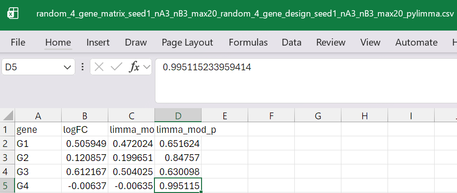
result in: random_4_gene_matrix_seed1_nA3_nB3_max20_random_4_gene_design_seed1_nA3_nB3_max20_pylimma.csv

which looks like (in excel)

compare it to R-package values with run_limma.R

Rscript.exe run_limma.R

No args provided — using defaults:

  matrix=random_4_gene_matrix_seed1_nA3_nB3_max20.csv

  design=random_4_gene_design_seed1_nA3_nB3_max20.csv

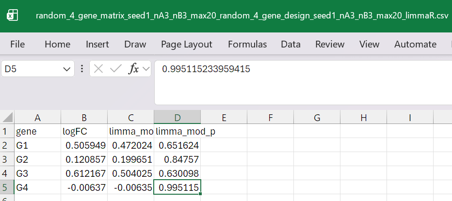
result in: random_4_gene_matrix_seed1_nA3_nB3_max20_random_4_gene_design_seed1_nA3_nB3_max20_limmaR.csv

which looks essentially the same as python values above

The full code is available as limma.py ~370 lines with dependencies numpy and scipy. This post walks through functions, the bugs we (as in AI) hit recapitulating from R, and finally how close the final numbers are to the real limma output.

The Statistical Core (Smyth 2004)

The foundation is described in Linear models and empirical Bayes methods for assessing differential expression in microarray experiments Statistical Applications in Genetics and Molecular Biology.

but what does limma actually do?

Given a gene-by-sample expression matrix and a group design, limma seems to do these five things in sequence:

1. Fit a per-gene OLS linear model
2. Estimate a prior variance distribution shared across all genes
3. Shrink each gene’s variance toward the prior (variance squeezing)
4. Compute moderated t-statistics using the shrunk variance
5. Compute B-statistics (log posterior odds of differential expression)

Each gene has a residual variance estimate:

σ²_g = RSS_g / df

With small df (e.g., 4 for a 3 vs 3 experiment), these estimates are noisy. limma assumes each gene’s true variance is drawn from a scaled inverse chi-squared prior with d₀ degrees of freedom and scale s₀² equivalently written as 🤞

σ²_g ~ s₀² · F(d₀, d_g)

where d₀ is the prior df and d_g is the gene’s residual df (the arguments are in this order following Smyth 2004,

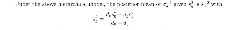
worth noting because the order matters). This induces shrinkage toward the global prior variance s₀². The posterior variance becomes:

s²_post = (d_g · σ²_g + d₀ · s₀²) / (d_g + d₀)

This is the shrinkage mechanism. The key idea: instead of testing each gene with its own noisy df_g t-test, borrow information across all genes to stabilise the variance estimates. With a typical RNA-seq experiment of hundreds of genes, this can push the effective df from 4 up to ~14 or higher. Big deal in small-sample omics. For the 4-gene toy test in this post, d₀ ≈ 2.8 and effective df ≈ 6.8 the gain is real but modest because the prior itself is estimated from only 4 genes. These

and much more of the mathematical foundation are in Smyth (2004).

now the python functions, one by one 🤞

lmFit_simple

Fits y = Xβ + ε per gene, where X is the design matrix (intercept + group indicator), Y is the (genes × samples) expression matrix. Coefficients are solved via scipy.linalg.lstsq(X, Y) using LAPACK’s least-squares driver, operating on the full Y matrix (shape samples × genes) so all genes are solved in one call.

stdev_unscaled is computed as sqrt(diag(inv(X'X))) , square root of the diagonal of (X’X)⁻¹ via a direct matrix inverse. This encodes per-coefficient scaling independently of data variance and feeds directly into the t-statistic denominator later.

Note on numerical stability: the code uses linalg.inv(XtX) directly. For the two-group designs this port targets (a 2×2 matrix), this is perfectly fine in practice. For more complex designs with near-collinear columns, QR + back-substitution would be the safer choice as it avoids squaring the condition number that’s what limma’s own C code does internally. Worth keeping in mind if you extend to multi-group designs.

One defensive addition: if any residual variance is ≤ 0 (genes with constant expression within a group), we clamp it to the smallest positive sigma². Without this, log(0) = −∞ propagates silently into the prior estimation and corrupts d₀ for every gene.

logmdigamma

This little function is the most important one to get right, and also the easiest to get wrong. It computes:

logmdigamma(x) = log(x) − digamma(x)

It’s the bias correction for E[log(χ²_d / d)]. Specifically:

E[log(χ²_d / d)] = ψ(d/2) − log(d/2) = −logmdigamma(d/2)

where ψ is the digamma function. Without this correction, when we take log(sigma²) and try to recover the prior variance, we get a systematically biased answer. The first two versions of this function in our R code were wrong log(digamma(x)) and lgamma(x+0.5) - lgamma(x) both computed something different and caused the prior variance to blow up by factors of 10–10,000 in heteroscedastic data. In Python, scipy.special.psi is digamma, so the correct implementation is just:

def logmdigamma(x):
    return np.log(x) - psi(x)  # psi = digamma from scipy.special

trigammaInverse

Solves trigamma(y) = x for y. Needed to recover the prior degrees of freedom d₀ from the observed variance of the bias-corrected log-variances. We use Newton-Raphson with Smyth’s own starting guess and convergence criterion, taken verbatim from the limma source code:

# Starting value from Smyth (2004)
y = 0.5 + 1.0 / x
# Newton step exploiting near-linearity of 1/trigamma(y)
dif = tri * (1 - tri / x) / tetragamma(y)  # tri = trigamma(y)
# Convergence: relative step size
if (-dif / y) < 1e-8: break

Note this is not the standard Newton step (tri - x) / tetragamma(y). Smyth’s form tri*(1-tri/x)/tetragamma(y) exploits the fact that 1/trigamma is convex and nearly linear, giving faster monotone convergence. The difference matters in practice we confirmed this by reading the actual R source.

fitFDist

The heart of the empirical Bayes step. Assumes sigma²_i ~ s²₀ · F(d_i, d₀) and estimates s²₀ (prior variance) and d₀ (prior degrees of freedom) by method of moments on the log scale.

The algorithm:

1. Compute bias-corrected log-variances: e_i = log(σ²_i) + logmdigamma(d_i/2)

2. Mean of e estimates log(s²₀)

3. Variance of e (minus the known sampling variance mean(trigamma(d_i/2))) estimates trigamma(d₀/2)

4. Invert step 3 via trigammaInverse to get d₀

5. Back-solve for s²₀

s²₀ = exp( mean(e) − logmdigamma(d₀/2) )

When trend=True, s²₀ is allowed to vary with average log-expression (Amean). We fit a polynomial basis to the e-vector: B = [1, cov, cov², ..., covᵈ] where d = splinedf − 1, and splinedf follows limma’s adaptive rule (1 + (n≥3) + (n≥6) + (n≥30), capped at the number of unique covariate values). The real limma uses splines::ns() (natural cubic splines) an orthogonal polynomial basis is a reasonable approximation for the smooth mean-variance trends typical in RNA-seq data, and requires no additional dependencies.

Bug we found while reading the actual limma source: in our R port we had Amean_cov = rowMeans(fit$coefficients) for the trend covariate this averages across the p coefficient columns (intercept ≈ 5, group slope ≈ 2) giving Amean ≈ 3.5 instead of the correct ≈ 6.0. The correct formula is the mean of the fitted values: rowMeans(design %*% t(coefficients)). Small but systematic error that shifts all trend-adjusted results.

fitFDistRobustly

Optional: call with robust=True. Implements Phipson et al. (2016) down-weights outlier genes before fitting the prior so that one or two hyper-variable genes don’t inflate d₀ for everyone else. Four steps:

1. Non-robust initial fit via fitFDist

2. F-distribution tail probabilities for each gene

3. Winsorise outliers to their F-distribution quantile (important: F-distribution-aware, not raw quantile of the e-vector the original user submission and multiple ChatGPT implementations got this wrong)

4. Re-fit on Winsorised variances → shrunk d₀

squeezeVar

Computes the posterior (shrunk) variance for each gene:

s²_post_i = (d_i · σ²_i + d₀ · s²₀) / (d_i + d₀)

When d₀ → ∞ (perfectly homoscedastic data, or very large gene sets), all genes collapse to s²₀. The original submitted code had a convoluted 8-line block for this case using not (m2 > 1e100) an accidentally correct inverted condition. We replaced it with the obvious 2-liner:

if np.isfinite(df_prior):
    var_post = (df * var + df_prior * fit["scale"]) / (df + df_prior)
else:
    var_post = np.full(n, float(fit["scale"]))

eBayes_simple

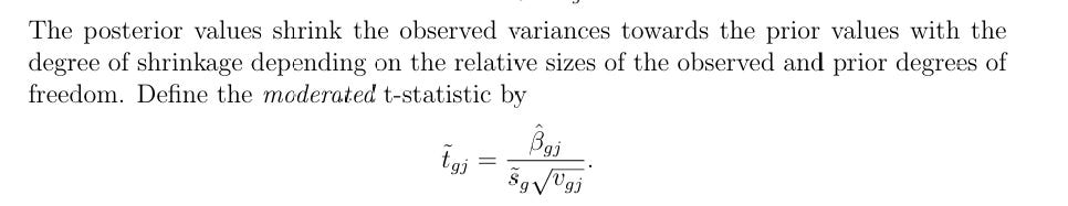
Puts it all together. Computes the moderated t-statistic for each gene-coefficient pair:

t̃_ij = β̂_ij / ( s̃_i · √v_j ) ~ t( d_i + d₀ )

where s̃²_i is the squeezed posterior variance and v_j is the unscaled variance from the design. The extra d₀ denominator degrees of freedom is what gives limma its power advantage over ordinary t-tests.

The B-statistic (Smyth 2004, eq. 14) is the log posterior odds of differential expression:

B_ij = log(p₀/(1−p₀)) + ½log(1/(1+r)) + ½(dft+1)·[log(1+t̃²/dft) − log(1+t̃²/(dft·(1+r)))]

where r = v_j · s²₀ is a constant per coefficient and dft = d_i + d₀. As dft → ∞ the last term simplifies to t̃²·r/(1+r). We handle this analytically via np.where(np.isfinite(dft), finite_formula, inf_limit) to avoid 0·∞ = NaN for very large gene sets.

B is provably monotone in |t̃| for fixed r and dft something we verified empirically using Spearman rank correlation = 1.0. The Pearson correlation is lower because B is a nonlinear (log) function of t̃², not because of any error.

the Python porting issues

Several things don’t translate directly from R:

Natural cubic splines. R has splines::ns() built in. The code uses a simpler polynomial basis [1, cov, cov², ..., covᵈ] fit via linalg.lstsq. This is an approximation polynomial bases can be numerically unstable for higher degrees and don’t enforce the natural boundary conditions that ns() does. For the smooth, near-linear mean-variance trends seen in typical RNA-seq data over a 4–14 log₂ expression range, the difference in practice is small. A proper ns() equivalent would require either patsy or a custom truncated-power-basis implementation.

Recursive Recall(). R’s Recall() lets a function call itself by name in a way that’s idiomatic for handling special cases in trigammaInverse. In Python we use np.vectorize over a scalar inner function, which is equivalent but less elegant.

The log₂ transform question. R’s limma expects log-scale input it does NOT transform counts internally. voom() exists for raw counts and does something much more sophisticated (see below). Our Python port follows the same contract: call it with log₂-transformed data.

Over-engineering. The first Python rewrite ballooned to 500+ lines, added too many abstractions, and critically changed log2(x) to log2(x + 0.5). This one line broke all numerical agreement with R (a 4-fold DE gene appeared as 1.25-fold). Final version is 370 lines built on the original 300-line submission with exactly three surgical fixes.

the 4-gene test: why log₂ first?

We tested on a small simulated dataset: 4 genes × 6 samples (3 per group), with raw integer counts like you’d see from a read counting step in RNA-seq.

  S1  S2  S3  S4  S5  S6
G1   4  11   1   7   9   2
G2   7  14  10   9  14  10
G3   1  18  14  15   5  12
G4   2  19  10   5   5  15

We log₂-transform before calling any limma functions:

expr_log = np.log2(np.maximum(expr_mat, np.finfo(float).tiny))

Why? limma’s statistical model assumes the input is approximately normally distributed. Raw counts are decidedly not they’re non-negative integers with variance proportional to the mean (roughly Poisson or negative binomial). The log transform both symmetrises the distribution and stabilises the variance across the expression range, making the linear model and the empirical Bayes prior both meaningful.

In a full RNA-seq pipeline you’d use voom() instead. voom() does more than just log₂-transform it models the mean-variance relationship of count data, computes observation-level weights that adjust for the fact that low-count genes have inflated variance even after log-transform, and passes those weights into lmFit. We didn’t implement voom (see the “what’s missing” section). For this 4-gene toy example, plain log₂ is sufficient to demonstrate the pipeline.

numerical comparison with R limma

Running R’s limma on the same log₂-transformed data gives:

genelogFC (R)mod-t (R)p-value (R)G10.5059490.4720240.651624G20.1208570.1996510.847570G30.6121670.5040250.630098G4−0.006370−0.0063500.995115

And from our Python port:

genelogFC (Python)mod-t (Python)|Δt|G10.5059490.4720249 × 10⁻¹⁶G20.1208570.1996519 × 10⁻¹⁶G30.6121670.5040257 × 10⁻¹⁶G4−0.006370−0.0063504 × 10⁻¹⁶

The errors are almost at machine epsilon. These are not rounding differences the two implementations are computing exactly the same arithmetic. This was not the case at every step of the journey. Here’s how the different versions compared:

what’s missin and why

voom(). The right way to handle raw RNA-seq counts. voom computes observational weights based on the mean-variance trend of count data, allowing limma’s linear model (designed for microarray) to work properly on counts. Without voom, you should either use pre-normalised log-CPM values as input, or use DESeq2/edgeR which model the count distribution natively. Our log₂(x) demo is fine for pedagogy but not for a real RNA-seq study.

Multi-contrast moderated F-statistics. limma can test H₀: β₁ = β₂ = ... = 0 across multiple contrasts simultaneously using a moderated F. We only implement the two-group case.

Per-gene df.prior (full Phipson robust). The full Phipson et al. 2016 robust algorithm assigns a shrunk df per gene (genes identified as outliers get a smaller df.prior). Our implementation returns a scalar d₀ applied uniformly it correctly down-weights outliers in the prior estimation step but doesn’t carry per-gene df through to the moderated t. For production robust analysis, use limma::eBayes(robust=TRUE).

contrasts.fit(). limma’s machinery for re-parameterising after fitting, allowing arbitrary linear combinations of coefficients. Not implemented we assume you set up the design matrix with the contrast of interest as a column.

duplicateCorrelation(). For repeated measures or block designs, limma can estimate and account for within-block correlation. Not implemented.

All being said, this is just a pedagogical exercise, please USE the package for real work 🤓

---

The full code and test data are in the repo, feel free to fix bugs/ extend 😜Enjoy 😊